LAURA T. STARKS, LI YONG and LU ZHENG∗
THE JOURNAL OF FINANCE • VOL. LXI, NO. 6 • DECEMBER 2006
ABSTRACT
This paper provides direct evidence supporting the tax-loss selling hypothesis as an explanation of the January effect. Examining turn-of-the-year return and volume patterns for municipal bond closed-end funds, which are held mostly by tax-sensitive individual investors, we document a January effect for these funds, but not for their underlying assets. We provide evidence that this effect can be largely explained by tax-loss selling activities at the previous year-end. Moreover, we find that funds associated with brokerage firms display more tax-loss selling behavior, suggesting that tax counseling plays a role.
AMONG THE NUMEROUS STOCK RETURN ANOMALIES, probably none has generated more interest than that of the “turn-of-the-year” or “January” effect, the phenomenon in which small capitalization stocks realize unusually high returns in early January.1 The literature offers a number of hypotheses to explain this phenomenon including the tax-loss selling hypothesis, the window dressing hypothesis, the insider trading (information release) hypothesis, and the seasonality of the risk–return relation hypothesis. Given existing evidence in some support for the first two hypotheses, the debate continues with respect to which of these, the tax-loss selling of individual investors or the window dressing of institutional investors, is the main driver of the turn-of-the-year effect.2 In this paper, we provide direct evidence in support of the tax-loss selling hypothesis by examining the trading and return patterns of municipal bond closed-end funds, which are held primarily by tax-sensitive individual investors.
The tax-loss selling hypothesis has been the most frequently cited explanation for the January effect since Branch (1977), who documents high January returns for stocks that incur negative returns during the previous year. Specifically, the hypothesis posits that shortly before year-end, investors sell securities in which they have losses in order to lower their taxes on net capital gains. Thus, while intensified selling pressure depresses prices at yearend, the prices rebound in January, resulting in large January returns. Empirical tests of the tax-loss selling hypothesis provide mixed results. On the one hand, Dyl (1977), Givoly and Ovadia (1983), and Reinganum (1983) show that stocks declining in price tend to record abnormally high volume in December and abnormally high returns in January.3 On the other hand, research also provides evidence that is somewhat counter to tax-loss selling as an explanation of the January effect. For example, Constantinides (1984) indicates that the optimal tax trading strategy is not to delay loss realization until December, Reinganum (1983) shows that nondeclining small firm stocks also record abnormally high January returns, Van den Bergh and Wessels (1985) demonstrate that the January effect obtains in markets without capital gains taxes, and Jones, Pearce, and Wilson (1987) report that the January effect obtains even before the imposition of income taxes in the United States.4
The leading alternative explanation for the January effect is the institutional investor window dressing hypothesis of Haugen and Lakonishok (1988). According to this hypothesis portfolio managers sell losing issues before a period ends in order to avoid revealing that they have held poorly performing stocks. Evidence that is generally consistent with the window dressing hypothesis exists in markets for instruments that are held primarily by institutional investors. For example, Musto (1997) finds a turn-of-the-year effect among money market instruments. Because these instruments do not generate capital losses, that is, tax effects, Musto concludes that at least some of the January effect in the equity market represents window dressing by portfolio managers and not tax-loss selling. Similarly, Maxwell (1998) concludes that window dressing is a significant factor behind the January effect in non investment grade bonds.5 Ritter and Chopra (1989) and Meier and Schaumburg (2004) also provide evidence consistent with the window dressing hypothesis.
Because many of the predictions of the window dressing and tax-loss selling hypotheses are the same, it is difficult to determine which explanation, if either, drives the January effect. For instance, Sias and Starks (1997) and Poterba and Weisbenner (2001) both design controlled tests to disentangle and separately evaluate the two hypotheses in the equity market, and both of these studies find evidence that is more consistent with the tax-loss selling hypothesis.6 However, the inability to distinguish institutional trades from individual trades or to distinguish tax-motivated trades from other trades makes their results suggestive but incomplete, as neither study is able to completely control for the potential existence of window dressing effects.
Our study is most closely related to previous studies that test (and support) the tax-loss selling hypothesis through examinations of individual investor
trades (e.g., Badrinath and Lewellen (1991), Dyl and Maberly (1992), Grinblatt and Keloharju (2001), Odean (1998), Ritter (1988, 2004), and Ivkovic, Poterba, and Weisbenner (2005)). Using this approach, the authors examine trades on all types of stocks and they infer tax-loss selling by examining the effects of previous stock returns on the year-end trades and, in turn, on the subsequent January returns. In this paper, in contrast, we examine the turn-of-the-year effect in a setting in which it is less difficult to isolate the trades of tax-sensitive individual investors. Specifically, we examine the trading and return patterns of a class of securities that are held almost exclusively by individual investors particularly sensitive to taxes, namely municipal bond closed-end funds. To the extent that tax-loss selling explains the January effect in the equity markets in general, we should observe a similar or stronger effect in municipal bond closed end funds because investors in these funds are among the most tax sensitive by self-selection, and thus they are more likely to sell on losses for tax reasons.7 Evidence of a January effect in municipal bond closed-end funds would therefore provide a more direct link between turn-of-the-year price effects and tax-loss trading activity.
Two additional features of municipal bond closed-end funds are important for our purposes. First, unlike open-end funds, closed-end funds trade like stocks. As a result, we are able to observe any price effects of trading activity as well as patterns in trading volumes. Second, given municipal bond closed-end funds were introduced in the 1990s, they are a relatively new set of securities. Thus, we encounter less ambiguity regarding the tax basis of investors (that is, differences with respect to when securities are purchased) than do studies of the tax effects of most equity shares. In a recent study, Elton, Gruber, and Blake (2004) also exploit some unique features of municipal bond closed-end funds and provide support for the tax explanation of ex-dividend day behavior.
Using a sample of 168 municipal bond closed-end funds over the 1990 to 2000 sample period, we first document that the average January return for municipal bond closed-end funds is 2.21%, which is significantly higher than the average return of −0.19% for the other 11 months of a year. Moreover, our empirical results indicate that there exists a direct link between the observed January price effect and the tax-loss selling behavior of individual investors at year-end. Specifically, in cross-sectional and panel analyses of the closed-end funds, we find that the January abnormal returns are positively related to the previous year-end volume measures, and in turn the year-end volume measures are negatively related to past fund returns. Year-end volume is significantly larger in years in which fund prices have declined. Moreover, losses appear to have an effect on the subsequent year-end trading volumes if funds do not regain their previous prices. We also find that January and December buy–sell ratios are significantly related to returns in a manner consistent with the tax-loss selling hypothesis.
In additional analysis that is unique to tests of the tax-loss selling hypothesis, we examine whether brokers play a role in investors selling on losses. We hypothesize that brokers have incentives to recommend such strategies because of their roles as financial advisers and because of the commissions that tax-loss selling generates. We therefore predict that fund investors who have access to brokerage advice, and presumably tax counseling, display more tax-loss selling behavior than those who do not. We find that, indeed, funds associated with brokerage firms are more likely to record year-end tax-loss selling, suggesting that brokerage firms advise their clients to engage in tax-motivated trading.
In summary, we find that the January effect in municipal bond closed-end fund prices is largely explained by the tax-loss selling behavior of fund investors at the turn of the year. Thus, our findings provide new evidence in support of the tax-loss selling hypothesis in explaining the January effect.
The remainder of the paper is organized as follows. Section I describes the data. Section II presents the empirical results that relate to turn-of-the-year effects. Section III provides results regarding the effects of tax counseling by brokers. Section IV concludes.
I. Data
The principal data for this study come from the Center for Research in Security Prices (CRSP) monthly stock files. For each year from 1990 to 2000, we
obtain prices, shares outstanding, monthly volumes, and monthly returns (including and excluding dividends) for a sample of 168 municipal bond closed-end funds (most of which were established in the early- to mid-1990s). Because dividends on municipal bond closed-end funds are tax-exempt but price changes are not, tax-loss selling behavior should be driven by the price changes only. We report the test results using the return series excluding dividends; however, the empirical results are very similar in terms of magnitude and significance if we use returns including dividends. We obtain the fund categorization from CDA/Wiesenberger and the monthly returns on a proxy for the underlying assets, a municipal bond index, from Ibbotson Associates.
The first municipal bond closed-end fund was established in 1986. These funds became popular in the early 1990s for several reasons: (1) effective tax
rates were increasing and 1986 tax law changes had removed other methods of sheltering money from taxes; (2) interest rates were falling and investors were looking for higher yields; and (3) most of these funds were leveraged to produce higher tax-exempt yields (Gould (1992a, 1992b)). Laing (1987), Quinn (1987), and Siconolfi (1987) discuss the tax advantages of holding of these funds further. The number of funds therefore grew rapidly in the early 1990s. Our sources indicate that there were 17 such funds in 1990, 62 in 1993, and 140 in 1995. By 2000 there were 165 municipal bond closed-end funds. Three funds went defunct during our sample period.
II. Empirical Results: Turn-of-the-Year Effects
A. The January Effect in Municipal Bond Closed-End Funds
To test for a January effect among municipal bond closed-end funds, for each month over the 1990 to 2000 time period we calculate the average return across all funds with data available. Figure 1 shows the time-series average returns for each of the 12 months in a year. The average return in January is 2.21%, as compared to an average of −0.19% across the other 11 months.
Using a simple time-series regression of cross-fund average returns on a January dummy variable, we find, again, that the return is significantly higher (at the 1% level) in January than in the other months. The regression results, which we report in Table I, show that the average return in January is about 2.4% higher than the average return across the other months. In a second regression, which we also report in Table I<< we include the monthly returns on the municipal bond index. Even after controlling for the municipal bond index returns, the average return in January still exceeds the average return in the other months by 2.17%, significant at the 1% level. This finding indicates that the observed January effect is not due to return seasonality in the underlying municipal bond index, which may be viewed as a proxy for the Net Asset Value (NAV) of the closed-end funds. In fact, as the last regression in the table shows, the return on the municipal bond index does not display the January seasonal pattern for the sample period from 1990 to 2000.
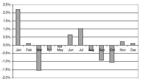
Figure 1. Average monthly return of the muni bond funds for the 12 calendar months.
The figure shows the average return across all municipal bond closed-end funds with data available for each of the 12 months in a year during the 1990–2000 time period.
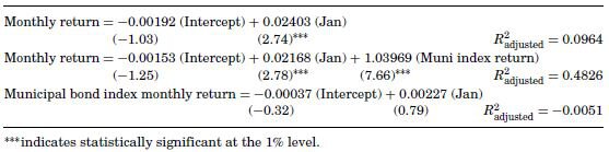
Table I. Regressions of Monthly Returns on January Dummies
This table presents three regressions of monthly returns. Model (1) shows results of regressions of monthly returns against monthly dummy variables. Model (2) is the same regression but augmented with a control for monthly municipal bond index returns. Model (3) is a regression of the monthly
municipal bond index return against the monthly dummy variables. The table shows only the estimated coefficients for the January dummy variables along with the accompanying t-statistics and the regression R2s. All t-statistics are based on the Newey–West (1987) heteroskedasticity and autocorrelation consistent standard errors (t-statistics in parentheses). The coefficients for the other months, not shown, are never significantly different from zero at the 5% level.
Several potential explanations exist for why we observe a significant January effect in the municipal bond closed-end funds, but not in the underlying municipal bonds. First, the majority of municipal bond closed-end funds are leveraged. Thus, when losses occur in the underlying municipal bonds, the closed end funds’ losses are magnified by the leverage, which increases the incentives for fund shareholders to take advantage of tax-loss selling. Second, the holders of closed-end funds consist almost entirely of individual investors, whereas the holders of municipal bonds consist largely of institutional investors. For example, in the third quarter of 2000, only about 34.2% of the direct holders of municipal bonds were individual investors and an additional 6.7% were trusts and estates (which are individually taxed); the remaining municipal bond holders were institutions-–open-end mutual funds (14.7%), closed-end funds (4.6%), tax-exempt money market funds (14.7%), insurance companies (14.2%), commercial banks (7.3%), and assorted corporate accounts, brokers, and dealers.8 These ownership patterns are important because institutional holders of municipal bonds do not have the same incentives to engage in tax-loss selling as do individual investors. For instance, the compensation of open-end and closed-end fund managers is usually based on total return performance rather than after-tax return performance. Moreover, money market funds hold only short-term municipal bonds, and they do not tend to trade securities once they have been purchased. Thus, these types of institutional investors would be less inclined to sell off their municipal bond holdings due to tax-loss considerations.
The differences we find in Table I for the turn-of-the-year effects between the municipal bond closed-end funds and their underlying assets also have
implications for the so-called closed-end fund puzzle (e.g., Berk and Stanton (2004), Brickley, Manaster, and Schallheim (1991), Lee, Shleifer, and Thaler (1990)). Specifically, the fact that tax-loss selling incentives can vary between the holders of the closed-end funds and the holders of the underlying assets suggests that these incentive differences provide an additional explanation for why such funds realize market prices that differ from their net asset values and result in a premium or discount.
B. January Abnormal Returns and Abnormal Year-End Volume
Under the tax-loss selling hypothesis shortly before year-end, investors sell securities in which they have losses in order to realize the tax benefits of the losses and prices for these securities rebound in January when such selling pressure dissipates. If tax-loss selling is the dominant explanation for the January effect, we should observe a positive correlation between January abnormal returns for the closed-end funds and the previous year-end volume measures. Although Constantinides (1984) argues that delaying tax-loss selling to the end of the year is not optimal, Badrinath and Lewellen (1991) find that most sales of losers occur in November and December. Further, Bhabra, Dhillon, and Ramirez (1999) document a November effect related to tax-loss selling. Thus, our year-end volume measures focus on both November and December volumes.
We use the following two measures for each fund (equation 1):

The first measure is turnover, which equals a fund’s average monthly trading volume in November and December divided by the number of fund shares outstanding at the beginning of the year. This measure controls for variation in the number of outstanding shares across funds. The second measure of year-end volume, the volume ratio equals a fund’s average monthly trading volume in November and December divided by the fund’s average monthly volume from February to October in the same calendar year. The volume ratio measures a fund’s year-end volume relative to that of the other months in the same year and therefore controls for fund-specific and time-specific fluctuations. For example, noise due to trends in the trading volume of individual funds is moderated by adjusting the year-end volume by the 9-month average. Both the turnover and volume ratio measures allow for comparisons across funds even when their normal trading volumes differ in magnitude.
Using these two volume measures as alternative independent variables, we estimate the regression equation where Janret is the return in January and ret2−10 is the average monthly holding period return from February to October in the preceding year (equation 2).
![]()
We estimate the abnormal returns in January by controlling for the previous February to October returns. Panel A of Table II provides the results for a panel regression. As the results demonstrate, regardless of which independent variable we employ, abnormal January returns are significantly positively related to the previous year-end trading volume. Further, the R2s indicate that a relatively large proportion of the abnormal January returns can be explained by the previous year-end trading activities. As a further test, rather than pooling the data, we run annual regressions of equation (1) and find results (not shown) that are consistent with the panel regressions. The coefficients on turnover and vol ratio are positive and statistically significant at the 5% level for 10 out of the 11 years.9,10
Previous studies find that most of the total January abnormal return occurs during the first several trading days of the month.11 To examine whether our previous test results are driven primarily by returns on the first trading days of January, we repeat the analysis of Table II, PanelAusing the first 5-day returns of January rather than the full-month returns. The results of this analysis, which we report in Panel B of Table II, are consistent with those of Panel A for the full month. Thus, we find evidence that trading activity at the end of the year can explain a significant proportion of the variation in the returns during the first 5 trading days of January, consistent with the implications of the tax-loss selling hypothesis.
Table II. Panel Regression of January Returns on Volume Measures
This table shows the coefficients from regressions of January returns, adjusted by the previous February through October average returns, against volume measures. Model (1) measures volume by turnover and Model (2) measures volume by the volume ratio. In Panel A the return is calculated
using all trading days in January. In Panel B the return is calculated using only the first five trading days of January. There are 144 cross sections and 11 years of data. All t-statistics are based on the panel corrected standard errors (PCSEs), which adjust for contemporaneous correlation, autocorrelation, and heteroskedasticity.

C. Tax-Loss Selling at Year-End
A further implication of the tax-loss selling hypothesis is that when funds experience negative returns in a year, they should exhibit significant increases in year-end trading volume, that is, tax-loss selling at year-end, and the increases in volume should be greater for funds that experienced greater price declines during the year. Thus, we regress year-end volume measures on the current and previous year’s returns as follows (equation 3):
![]()
where returnc is the current year return, which we define as the cumulative monthly return of holding that fund from January to October in that year, and returnp is the previous year return, which we define as the cumulative monthly holding period returns of the fund in the previous calendar year, from January to December.
Table III: Results for Panel Regression with Fixed Effects for Funds: Year-End Volume Measures on Current Year and Previous Year’s Returns
This table shows the coefficients from regressions of year-end volume measures on the current year and previous year returns, where current year returns are measured from February through October. Model (1) measures volume by turnover and Model (2) measures volume by the volume ratio. Coefficients on firm fixed effects and constants are not reported. There are 144 cross sections and 11 years of data. All t-statistics are based on the panel corrected standard errors (PCSEs), which adjust for contemporaneous correlation, autocorrelation, and heteroskedasticity.

In Table III, we report the results of the panel regressions with fund fixed effects.12 For both year-end volume measures, the coefficients on the current year and previous year returns are negative and significant at the 1% level, indicating a negative relation between the year-end volume and past fund returns. Further, the R2 values in these regressions are higher than 50%, indicating that past fund returns can explain a large proportion of the volume variation across the funds. These results provide substantial support for the hypothesis that tax considerations result in abnormal year-end trading volumes.13
Table III shows that year-end abnormal volume can be generally explained by the returns over the previous 2 years. During our sample period, there were several years in which the bond markets realized negative returns, which allows for further analysis. As Figure 2 shows, in 3 of the 11 years of our sample, the average annual return is negative: around −3%, −20%, and −22% in 1990, 1994, and 1999, respectively.14
Figure 2. Average annual return of the muni bond funds, 1990–2000.
The figure shows the average annual return across all municipal bond closed-end funds with data available during the 1990 to 2000 time period.
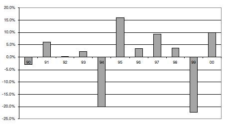
Figure 3 shows the average monthly fund turnover over the sample period, where we calculate average monthly turnover by summing the turnovers of all available funds in that month and dividing by the number of funds.
Comparing the return time series in Figure 2 to the turnover time series in Figure 3, we find that, in each of the 3 years with negative returns, the yearend turnover is larger than in the other years of the sample period. The pattern is most prominent in 1994 and 1999, when the municipal bond funds experienced the largest losses. Further, in the years subsequent to the large loss years, that is, in 1995, 1996, and 2000, the year-end turnover is still higher, most likely due to a lag effect in the selling of the fund shares. Indeed, the losses in 1994 and 1999 are so large that, on average, the funds do not regain their previous prices in the subsequent years of 1995 and 2000 (as can be seen from Figure 2) and thus investors can continue to realize accrued capital losses in these subsequent years. Interestingly, even in the subsequent years, the shareholders do not appear to sell until year-end.
Figure 3. Average monthly turnover of the muni bond funds, 1990–2000.
The figure shows the average monthly turnover across all municipal bond closed-end funds with data available during the 1990 to 2000 time period. A fund’s turnover is defined as its trading volume divided by the total number of shares outstanding at the beginning of the month.

To examine the relations between year-end volume and fund returns further, we also estimate annual cross-sectional regressions of equation (2).
Table IV reports the coefficient estimates and their corresponding t-statistics. Using turnover (the volume ratio) as the dependent variable, we find a significantly negative coefficient on the current year return in 7 (8) of the 11 years. Furthermore, the negative relation between the year-end volume and the current year return is most prominent in 1994 and 1999, when funds experience the largest losses. The negative relation between the year-end volume and the previous year return is strongest in 1995 and 2000, which is consistent with a lagged tax-loss effect.
Although these results support the tax-loss selling hypothesis as an explanation of the turn-of-the-year effect, they do not provide an explanation of why investors wait until the end of the year to effect these transactions nor why they wait until the end of the following year. Badrinath and Lewellen (1991) suggest that beyond reflecting lethargy in tax planning and transactions costs, the delay until the year-end may also represent investors not resolving their uncertainty about marginal tax rates or whether losses can be written off against long- or short-term capital gains until year-end. Based on their evidence, they argue that investors consider the turn-of-the-year to be an important tax planning event.
D. December and January Buy–Sell Ratios
If tax-loss selling is the dominant explanation for the abnormal December and January trading volumes, then we should observe differences in the buy–sell ratio around the year-end and this ratio should be related to both the current January return and the previous year’s return. To construct a ratio of apparent buy-to-sell volume for the turn-of-the-year period, we use the intraday trade and quote data from TAQ for the 1993 through 2000 period and we classify individual trades as market buy or market sell orders following the algorithm proposed by Lee and Ready (1991).15 Using the resulting buys and sells, we aggregate the buy volume and sell volume for the last 5 days in December and the first 5 days in January for each fund and we construct the fund’s average buy–sell ratios for those periods.
Table IV: Regression Results for Year-End Volume Measures on Current Year and Previous Year’s Returns
This table shows the coefficients from annual regressions of year-end volume measures on the current year and previous year returns, where current
year returns are measured from February through October. Model (1) measures volume by turnover and Model (2) measures volume by the volume ratio. All t-statistics are based on the Newey–West (1987) heteroskedasticity and autocorrelation consistent standard errors.

We find that just before year-end, the buy–sell ratio averages 0.85, which is significantly less than one (at the 1% level), indicating selling pressure at the end of the year. After the turn of the year, the buy–sell ratio averages 1.37, which is significantly greater than one (at the 1% level), indicating buying pressure at the beginning of the year. We also find that these January and December buy–sell ratios are significantly different from each other (at the 1% level).
Also consistent with the predictions of the tax-loss selling hypothesis, the three largest differences between the January and December buy–sell ratios occurred in the turn-of-the-year periods around 1994 to 1995, 1995 to 1996, and 1999 to 2000, which follow the large losses in the municipal bond markets in 1994 and 1999.
Table V provides the results of a panel regression of the December (January) buy–sell ratios against the current and previous years’ returns. The results show that the buy–sell ratio in the last few days of December is strongly related to the return over the previous February to October, as well as the return over the year preceding the current year. Municipal bond closed-end funds are sold more and/or purchased less at the end of the year when the returns over these periods are low. On the other hand, the buy–sell ratio in January is negatively related to the preceding returns: When funds have performed poorly, they are more likely to be associated with a higher buy–sell ratio in January, suggesting more reinvestment activities.
Although not shown in the table, we also examine whether the January 5-day return and January 5-day buy–sell ratio are related. As would be expected given our previous evidence, a strong relation exists between the return and the buy–sell ratio with a positive coefficient at a probability level of 0.0001, providing further evidence that the abnormal return in early January can be partly explained by the abnormal purchasing activities.
In summary, we find evidence that investors sell on capital losses at the end of the year and buy tax-advantaged funds at the beginning of the year, possibly moving their investments from a fund with losses to a similar tax-advantaged fund. The December and January buy–sell ratios are related to the asset returns in a manner consistent with the tax-loss selling hypothesis.
III. Tax-Loss Selling and Brokerage Firms
Another implication of the tax-loss selling hypothesis is that investors who receive investment advice should be more likely to engage in tax-loss selling.
Following this rationale, we develop a further “brokerage” hypothesis, which has not been examined in previous analyses of the January effect. We posit that closed-end funds held by investors who have an opportunity to receive more tax counseling should experience more tax-loss selling. Under this hypothesis, funds associated with a brokerage firm are more likely to engage in tax-loss selling because the brokers would presumably advise their client investors to take advantage of the tax benefits associated with realizing capital losses at year-end.
Table V: Results for Panel Regression with Fixed Effects for Funds: December Last 5-Day and January First 5-Day Buy-to-Sell Ratio on Current and Previous Years’ Returns
This table shows the coefficients from regressions of buy-to-sell ratios on the current and previous years’ returns, where current year returns are measured from February through October. The data cover the 1993 to 2000 period. There are 139 cross sections and 8 years of data. Coefficients
on the firm fixed effects and constants are not reported. All t-statistics are based on the panel corrected standard errors (PCSEs), which adjust for contemporaneous correlation, autocorrelation, and heteroskedasticity.

To test this hypothesis, we include a brokerage dummy variable that is equal to one if a closed-end fund management company is associated with a brokerage firm, and zero otherwise. We interact this dummy variable with the current and previous year returns. Table VI shows the fixed-effects panel regression results.16 The coefficients on the brokerage–return interaction terms are negative and significant at the 5% level for the current year’s return and in one specification for the previous year’s return. These results indicate that in addition to the negative return–volume relation, brokerage counseling is an important determinant of investor year-end tax-motivated trading activity. Thus, funds associated with brokerage firms display a stronger pattern of tax-loss selling at the end of the year, which supports the hypothesis that brokerage firms advise their clients to engage in tax-motivated trading. These results also suggest a new explanation for the tendency of tax-loss selling to occur at year-end: Investors receive tax planning advice from their financial advisors at year-end.
Table VI: Results for Panel Regression with Fixed Effects for Funds: Year-End Volume Measures on Current and Previous Years’ Returns with Brokerage Dummy and Interaction Terms Added
This table shows the coefficients from regressions of year-end volume measures on the current year and previous year returns, where current year returns are measured from February through October, and on these returns interacted with a dummy variable that is equal to one if the closed end
fund’s sponsor is also affiliated with a brokerage firm. Returnc D and Returnp D are the interaction terms between the brokerage dummy and the previous 2-year returns, respectively. Model (1) measures volume by turnover and Model (2) measures volume by the volume ratio.
Coefficients on firm fixed effects and constants are not reported. There are 144 cross sections and 11 years of data. All t-statistics are based on the panel corrected standard errors (PCSEs), which adjust for contemporaneous correlation, autocorrelation, and heteroskedasticity.

IV. Conclusion
The fact that municipal bond closed-end funds are held almost entirely by individual investors who are presumably tax sensitive makes them good candidates for the study of tax-loss selling as an explanation for the January effect. In this paper, we find evidence that the year-end tax-loss selling behavior of investors accounts for a large proportion of the January effect for this particular set of securities. In particular, we find that the abnormal returns of the municipal bond closed-end funds in January are positively correlated with the year-end trading volumes and that the year-end volumes are negatively related to the current and the previous year returns. Our findings support the tax-loss selling hypothesis. In addition, we find that closed-end funds associated with brokerage firms display more tax-loss selling behavior.
Our results show that during our sample period, a turn-of-the-year effect exists in the municipal bond closed-end funds but does not exist in the underlying municipal bonds. Although we do not examine the premiums or discounts on the funds, these results suggest an additional explanation for the closed-end fund puzzle: The tax status and time horizons of the holders of closed-end funds differ from those of the holders of the underlying assets. The question, then, is why the resulting price differential is not arbitraged away. A related question is why the January seasonality pattern is not arbitraged away, especially since it has been common knowledge for some years now. At least in the case of closed-end funds, the answer to both of these questions relates to the difficulty in entering into successful arbitrage positions. Pontiff (1996) identifies significant arbitrage costs for closed-end funds. In particular, he points out that due to their tax-exempt status, municipal bond closed-end funds cannot be sold short by arbitrageurs. Further, an investor may have difficulty replicating either a short or long position in the underlying municipal bonds because the holdings of the closed-end funds are not available in time, and even if they were, many municipal bonds are not widely traded.17
REFERENCES
Badrinath, S.G., and Wilbur G. Lewellen, 1991, Evidence on tax-motivated securities trading behavior, Journal of Finance 46, 369–382.
Banz, RolfW., 1981, The relationship between return and market value of common stocks, Journal of Financial Economics 9, 3–18.
Barber, Brad, and Terrance Odean, 2004, Are individual investors tax savvy? Asset location evidence from retail and discount brokerage accounts, Journal of Public Economics 88, 419–442.
Beck, Nathaniel, and Jonathan N. Katz, 1995, What to do (and not to do) with time-series cross section data, American Political Science Review 89, 634–647.
Bergstresser, Daniel B., and James Poterba, 2002, Do after-tax returns affect mutual fund inflows? Journal of Financial Economics 63, 381–414.
Bergstresser, Daniel, and J. Poterba, 2004, Asset allocation and asset location: Household evidence from the Survey of Consumer Finances, Journal of Public Economics 88, 1893–1915.
Berk, Jonathan, and Richard Stanton, 2004, A rational model of the closed-end fund discount, Working paper, University of California–Berkeley.
Bhabra, Harjeet, Upinder Dhillon, and Gabriel Ramirez, 1999, A November effect? Revisiting the tax-loss selling hypothesis, Financial Management 28, 5–15.
Blume, Marshall E., and Robert F. Stambaugh, 1983, Bias in computed returns: An application to the size effect, Journal of Financial Economics 12, 387–404.
Branch, Ben, 1977, A tax loss trading rule, Journal of Business 50, 198–207.
Brauer, Greggory A., and Eric C. Chang, 1990, Return seasonality in stocks and their underlying assets: Tax-loss selling versus information explanations, Review of Financial Studies 3, 255– 280.
Brickley, James, Steven Manaster, and James Schallheim, 1991, The tax timing option and the discount on closed-end investment companies, Journal of Business 64, 287–312.
Chan, K. C., 1986, Can tax-loss selling explain the January seasonal in stock returns, Journal of Finance 41, 1115–1128.
Chang, Eric C., and Michael J. Pinegar, 1986, Return seasonality and tax-loss selling in the market for long-term government and corporate bonds, Journal of Financial Economics 17, 391–415.
Constantinides, George, 1984, Optimal stock trading with personal taxes: Implications for prices and the abnormal January returns, Journal of Financial Economics 13, 65–89.
Dammon, Robert M., Chester S. Spatt, and Harold H. Zhang, 2001, Optimal consumption and investment with capital gains taxes, Review of Financial Studies 14, 583–616.
Dammon, Robert M., Chester S. Spatt, and Harold H. Zhang, 2004, Optimal asset location and allocation with taxable and tax-deferred investing, Journal of Finance 59, 999–1037.
Dyl, Edward, 1977, Capital gains taxation and year-end stock market behavior, Journal of Finance 32, 165–175.
Dyl, Edward, and Edwin Maberly, 1992, Odd-lot transactions around the turn of the year and the January effect, Journal of Financial and Quantitative Analysis 27, 591–604.
Elton, Edwin J., Martin J. Gruber, and Christopher R. Blake, 2004, Marginal stockholder tax effects and ex-dividend day behavior thirty-two years later, forthcoming, Review of Economics and Statistics.
Gallmeyer, Michael, Ron Kaniel, and Stathis Tompaidis, 2006, Tax management strategies with multiple risky assets, Journal of Financial Economics 80, 243–291.
Garlappi, Lorenzo, and Jennifer Huang, 2004, From location to allocation: Taxable and tax-deferred investing with portfolio constraints, Working paper, University of Texas at Austin.
Givoly, Dan, and Arie Ovadia, 1983, Year-end induced sales and stock market seasonality, Journal of Finance 38, 171–185.
Gould, Carole, 1992a, Mutual funds; popular closed-end municipals, New York Times (April 12), 18.
Gould, Carole, 1992b, Mutual funds; bargain look in closed-end munis, New York Times (July 12), 16.
Green, Richard, Burton Hollifield, and Norman Schurhoff, 2004, Financial intermediation and the costs of trading in an opaque market, Working paper, Carnegie Mellon University.
Grinblatt, Mark, and Matti Keloharju, 2001, What makes investors trade, Journal of Finance 56, 589–616.
Grinblatt, Mark, and Matti Keloharju, 2004, Tax-loss trading and wash sales, Journal of Financial Economics 71, 51–76.
Haugen, Robert, and Josef Lakonishok, 1988, The Incredible January Effect: The Stock Market’s Unsolved Mystery (Dow Jones-Irwin, Homewood, Illinois).
Huang, Jennifer, 2004, Taxable or tax–deferred investing: A tax-arbitrage approach, Working paper, University of Texas at Austin.
Ivkovic, Zoran, James Poterba, and Scott Weisbenner, 2005, Tax-motivated trading by individual investors, 95, 1605–1630, American Economic Review.
Jones, Charles, Douglas Pearce, and Jack Wilson, 1987, Can tax-loss selling explain the January effect? A note, Journal of Finance 42, 453–461.
Keim, Donald, 1983, Size-related anomalies and stock return seasonality: Further empirical evidence, Journal of Financial Economics 12, 12–32.
Laing, Jonathan R., 1987, Burnt offerings: Closed-end funds bring no blessings to shareholders, Barron’s August 10, 1987, 32–36.
Lakonishok, Josef, and Seymour Smidt, 1986, Volume for winners and losers: Taxation and other motives for stock trading, Journal of Finance 41, 951–974.
Lee, C., A. Shleifer, and R. Thaler, 1990, Anomalies: Closed-end mutual funds, Journal of Economic Perspectives 4, 153–164.
Lee, Charles M., and Mark J. Ready, 1991, Inferring trade direction from intraday data, Journal of Finance 46, 733–746.
Maxwell, William, 1998, The January effect in the corporate bond market: A systematic examination, Financial Management 27, 18–30.
Meier, Iwan, and Ernst Schaumburg, 2004, Do funds window dress? Evidence for U.S. domestic equity mutual funds, Working paper, Northwestern University.
Musto, David K., 1997, Portfolio disclosures and year-end price shifts, Journal of Finance 52, 1563–1588.
Newey, Whitney, and Kenneth West, 1987, A simple positive definite, heteroskedasticity and autocorrelation consistent covariance matrix, Econometrica 5, 703–705.
Ng, L., and Q.Wang, 2004, Institutional trading and the turn-of-the year effect, Journal of Financial Economics 74, 343–366.
Odean, Terrance, 1998, Are investors reluctant to realize their losses, Journal of Finance 53, 1775–1798.
Pontiff, Jeffrey, 1996, Costly arbitrage: evidence from closed-end funds, Quarterly Journal of Economics 111, 1135–1151.
Poterba, James M., and Scott J. Weisbenner, 2001, Capital gains tax rules, tax-loss trading, and turn-of-the-year returns, Journal of Finance 56, 353–368.
Quinn, J.B., 1987, Playing the closed-end funds, Newsweek August 17, 1987, 65.
Reinganum, Marc, 1983, The anomalous stock market behavior of small firms in January, Journal of Financial Economics 12, 89–104.
Ritter, Jay, 1988, The buying and selling behavior of individual investors at the turn of the year, Journal of Finance 43, 701–717.
Ritter, Jay, and Navin Chopra, 1989, Portfolio rebalancing and the turn of the year effect, Journal of Finance 44, 149–166.
Roll, Richard, 1983, Vas ist das? The turn-of-the-year effect and the return premia of small firms, Journal of Portfolio Management 9, 18–28.
Rozeff, Michael, and William Kinney, 1976, Capital market seasonality: The case of stock returns, Journal of Financial Economics 3, 379–402.
Seyhun, H. Nejat, 1988, The January effect and aggregate insider trading, Journal of Finance 43, 129–141.
Shoven, John B., and Clemens Sialm, 2004, Asset location in tax-deferred and conventional savings accounts, Journal of Public Economics 88, 23–38.
Sias, Richard W., and Laura T. Starks, 1997, Institutions and individuals at the turn-of-the-year, Journal of Finance 52, 1543–1562.
Siconolfi, M., 1987, Launching of closed-end funds may ease, Wall Street Journal November 27, 1987, 29.
Slemrod, Joel, 1982, The effect of capital gains taxation on year-end stock market behavior, National Tax Journal 35, 69–77.
Tinic, Seha M., and Richard R. West, 1984, Risk and return: January vs. the rest of the year, Journal of Financial Economics 13, 561–574.
Van den Bergh, W.M., and Roberto Wessels, 1985, Stock market seasonality and taxes: An examination of the tax-loss selling hypothesis, Journal of Business Finance and Accounting 12, 515–530.
Footnotes
1 Rozeff and Kinney (1976) first document the January effect, whereby stock returns are higher, on average, in January than in other months. Banz (1981) and Reinganum (1983) document that the effect is driven by smaller firms (measured by market capitalization), which realize higher average rates of return than do larger firms. While Keim (1983) reports that roughly half of the annual difference between the rates of return on small and large stocks over the 1963 to 1979 period occurs during the month of January, Blume and Stambaugh (1983) adjust Keim’s results for the “bid-ask spread” bias, and show that virtually all of the size effect occurs in the month of January. Roll (1983) dubs this interrelationship the “turn-of-the-year effect.”
2 Empirical evidence does not support the insider trading or risk-return seasonality hypotheses (Brauer and Chang (1990), Ritter and Chopra (1989), Rozeff and Kinney (1976), Seyhun (1988), Tinic and West (1984)).
3 Other studies that examine the tax-loss selling hypothesis include Slemrod (1982), Chan (1986), Lakonishok and Smidt (1986), Ritter (1988), and Dyl and Maberly (1992).
4 In addition, there exists considerable research on capital gain tax management strategies for investors. For recent research in this area, see, for example, Barber and Odean (2004), Bergstresser and Poterba (2004), Dammon, Spatt, and Zhang (2001, 2004b17), Garlappi and Huang (2004), Huang (2004), Shoven and Sialm (2004), and Gallmeyer, Kaniel, and Tompaidis (2005).
5 Chang and Pinegar (1986) find evidence of a January effect in noninvestment grade bonds, but no evidence of a January effect in investment grade bonds or in Treasury bonds.
6 Sias and Starks (1997) examine differences between securities dominated by individual investors versus those dominated by institutional investors and find that the effect is more pervasive in the former. Poterba and Weisbenner (2001) investigate the effect of specific features of the U.S. capital gains tax on turn-of-the-year stock returns and provide support for the role of tax-loss trading in contributing to the turn-of-the-year return patterns. See also Ng and Wang (2004) for institutional trading at year-end.
7 Bergstresser and Poterba (2002) document that money inflows of open-end mutual funds are affected more by after-tax returns than pre-tax returns.
8 Flow of Funds Accounts (Table L.211), published by Board of Governors of the Federal Reserve System (http://www.federalreserve.gov/releases/Z1/20001208).
9 All annual regressions report t-statistics based on the Newey–West (1987) heteroskedasticity and autocorrelation consistent standard errors.
10 As a further robustness test, instead of controlling for the previous February to October returns, we subtract from the January fund return the T-bill return for the same month. The results are similar in magnitude and significance to those in Panel A of Table II.
11 For example, see Keim (1983), Roll (1983), Ritter (1988), and Sias and Starks (1997).
12 The panel regressions include data from a total of 144 closed-end funds over 11 years. (We lose some fund observations because we require that each fund have complete return data for the previous 2 years.) The regressions use panel-corrected standard errors, which adjust for contemporary
correlation, autocorrelation, and heteroskedasticity (Beck and Katz (1995)).
13 Also consistent with the January effect, we estimate equation (2) with January volume measures and find results similar to those in Table III, but with coefficients that are smaller in magnitude.
14 We calculate the return for a year by compounding the average monthly returns.
15 According to this algorithm, trades are classified by comparing the transaction price to the prices of the prevailing quote, if available. Trades at the bid price are classified as sells and trades at the ask price are classified as buys. The prevailing quote is the current quote or the quote in effect 5 seconds ago if the current quote is less than 5 seconds old. Following Lee and Ready (1991), we only include quotes issued by the primary (NYSE) specialist and that are BBO-eligible, that is, eligible for inclusion in the NASD Best Bid and Offer calculation. When a BBO-eligible quote is unavailable or when a trade is at the midpoint of a spread, we use the “tick test” so that the trade is classified as a buy (sell) if the price change immediately before the trade is positive (negative). We classify trades inside the spread, but not at the middle of the spread, by their proximity to the bid or ask price—trades closer to the bid (ask) are classified as sells (buys). All trades except opening trades are included in the analysis.
16 Note that we do not list the dummy variable estimates in the table because they are picked up by the intercepts (fixed effects).
17 Green, Hollifield, and Schurhoff (2004) discuss the volume and the costs of municipal bond trading. They note that, according to the Municipal Securities Rulemaking Board (MSRB), 71% of outstanding issues did not trade at all from March 1998 to May 1999.
Note: In this report I have integrated the exact content of the original source, to be certain that this information is retained. If you would like to read this report on the website of the original publisher I recommend you to click the source link below.
Source: http://www2.mccombs.utexas.edu/faculty/laura.starks/starks%20yong%20zheng.pdf